Table of Contents
What are missing values in machine learning?
Missing values in a dataset indicate the absence of observations.
The danger of missing values
Why are missing values a problem for our job?
Missing values bring mainly 2 problems:
- Loss of information. We have less official and secure data on which to train our model.
- Missing values can introduce bias depending on their type (listed below). That’s because they can obscure important relationships between data.
Types of missing values
Missing completely at random (MCAR)
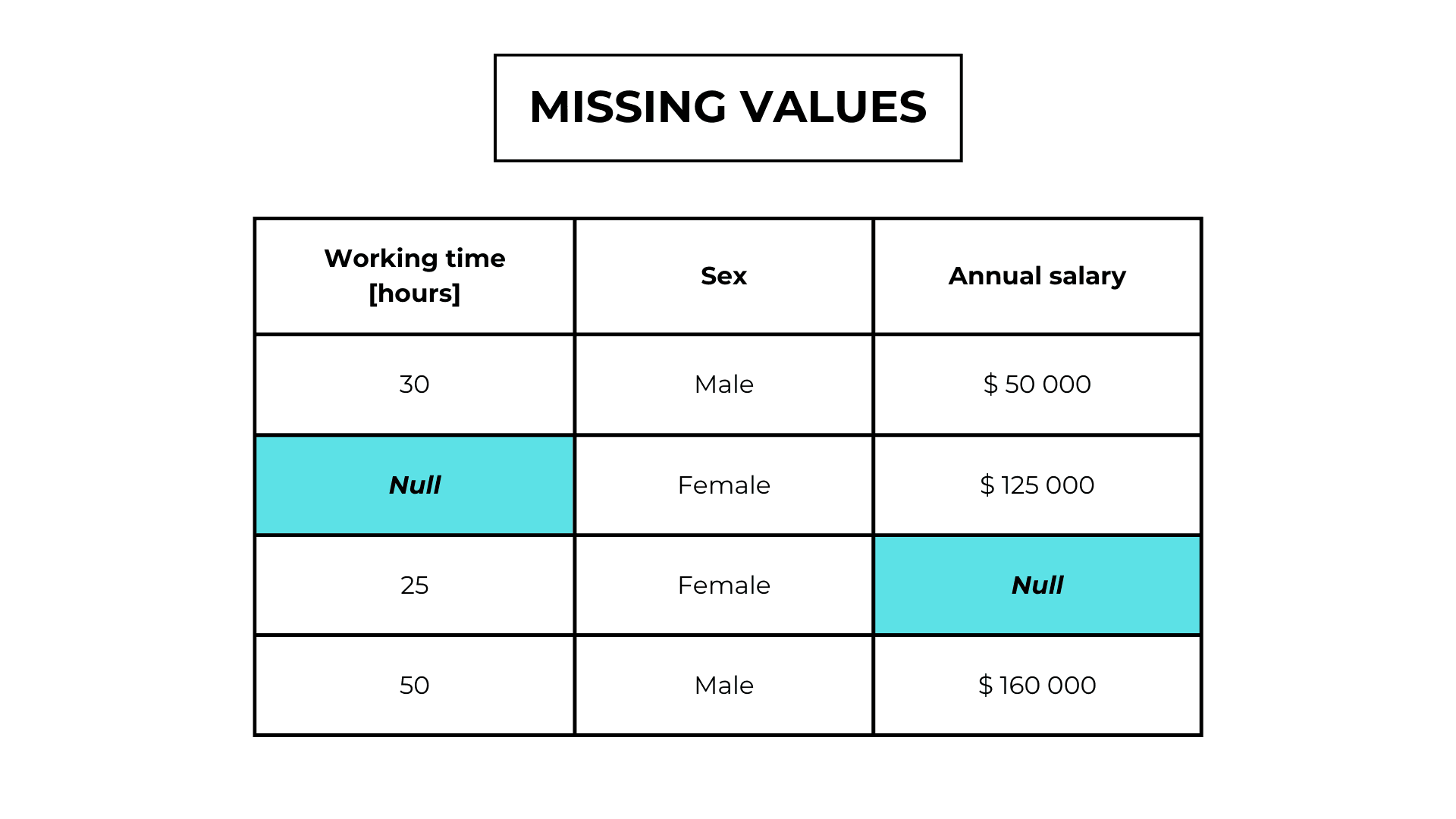
In Missing completely at random values, the missingness is independent of any other observation.
For example, someone forgot to answer a question in a survey or the system has a bug.
| Working time [hours] | Sex | Annual salary |
|---|---|---|
| 30 | Male | $ 50 000 |
| Null | Female | $ 125 000 |
| 25 | Female | Null |
| 50 | Male | $ 160 000 |
| 40 | Null | $ 60 000 |
| 50 | Female | Null |
Missing completely at random values are best for us because they don’t introduce any bias.
Missing at random (MAR)
In missing at random value, the missingness depends on observations of other features.
For example, in our dataset males are more reserved about their salaries than women.
| Working time [hours] | Sex | Annual salary |
|---|---|---|
| 30 | Male | Null |
| 40 | Female | $ 125 000 |
| 25 | Female | $ 30 000 |
| 50 | Male | $ 160 000 |
| 40 | Male | Null |
| 50 | Female | $ 85 000 |
Missing not at random (MNAR)
In missing not-at-random values, the missingness depends on the unobserved value itself.
For example, in our datasets, people with very high incomes may be more reserved.
| Working time [hours] | Sex | Annual salary |
|---|---|---|
| 30 | Male | $ 50 000 |
| 40 | Female | Null |
| 25 | Female | $ 30 000 |
| 50 | Male | Null |
| 40 | Male | $ 60 000 |
| 50 | Female | $ 85 000 |
How can we deal with missing values?
Drop observations
If an observation has got a missing value we remove it from the dataset.
| Working time [hours] | Sex | Annual salary |
|---|---|---|
| 30 | Male | $ 50 000 |
| 50 | Male | $ 160 000 |
| 50 | Female | $ 85 000 |
When to drop observation?
With this technique, we lose a lot of information. We should use it when the observations with missing values are 5% or less of the total samples.
Python implementation
X = pandas.DataFrame({
    "Area" : [30, 50, numpy.nan, 70, 25, numpy.nan],
    "PoolArea" : [10, numpy.nan, 5, 20, 15, numpy.nan]
})

new_X = X.dropna()
Drop features
We can delete an entire feature if it has too many missing values.
| Working time [hours] | Sex | Annual salary |
|---|---|---|
| 30 | Male | |
| 40 | Female | |
| 25 | Female | |
| 50 | Male | |
| 40 | Null | |
| 50 | Female |
When to drop a feature?
We should drop a feature when its number of missing values is 70-80% of the total.
Python implementation
X = pandas.DataFrame({
    "Area" : [30, 50, 15, 70, 25, 45],
    "PoolArea" : [10, 20, 5, 20, 15, numpy.nan]
})

null_columns = [column for column in X.columns if X[column].isnull().any()]

new_X = X.drop(axis=1, columns=null_columns)
Imputation
Imputation is a feature engineering technique for estimating missing values based on other observed values in the dataset.
Mean and median imputation
We replace each missing value in a feature with the mean (or median) value of the feature.
| Working time [hours] | Sex | Annual salary |
|---|---|---|
| 30 | Male | $ 50 000 |
| 34 | Female | $ 125 000 |
| 25 | Female | $ 98 750 |
| 50 | Male | $ 160 000 |
| 40 | Female | $ 60 000 |
| 50 | Female | $ 98 750 |
Python implementation
from sklearn.imputer import SimpleImputer

X = pandas.DataFrame({
    "Area" : [30, 50, numpy.nan, 70, 25, numpy.nan],
    "PoolArea" : [10, numpy.nan, 5, 20, 15, numpy.nan]
})

imputer = SimpleImputer(strategy="mean")

new_X = imputer.fit_transform(X)
When to use mean imputation?
Mean imputation is simple and effective for datasets where the missing data is random and the proportion of missing values is low.
Time-series data imputation
Last observation carried forward (LOCF)
We replace the missing value with the previous value in the feature.
| Time [years] | Cost |
|---|---|
| 1 | 20 |
| 2 | |
| 3 | 26 |
| 4 | 21 |
| 5 | 24 |
Python implementation
X = pandas.DataFrame({
    "Time" : [0, 1, 2, 3, 4, 5],
    "Value" : [60, numpy.nan, 80, 50, numpy.nan, 70]
})

new_X = X.fillna(method = "ffill")
Next observation carried backwards (NOCB)
We replace the missing value with the next value in the feature.
| Time [years] | Cost |
|---|---|
| 1 | 20 |
| 2 | |
| 3 | 26 |
| 4 | 21 |
| 5 | 24 |
Python implementation
X = pandas.DataFrame({
    "Time" : [0, 1, 2, 3, 4, 5],
    "Value" : [60, numpy.nan, 80, 50, numpy.nan, 70]
})

new_X = X.fillna(method = "bfill")
Interpolation
We estimate a missing observation by looking at the previous and next values.
This is the linear interpolation formula:
Where:
- y is the predicted value,
- x is the,
- x1 is the previous x value,
- x2 is the next x value,
- y1 is the previous y value,
- y is the target we want to predict
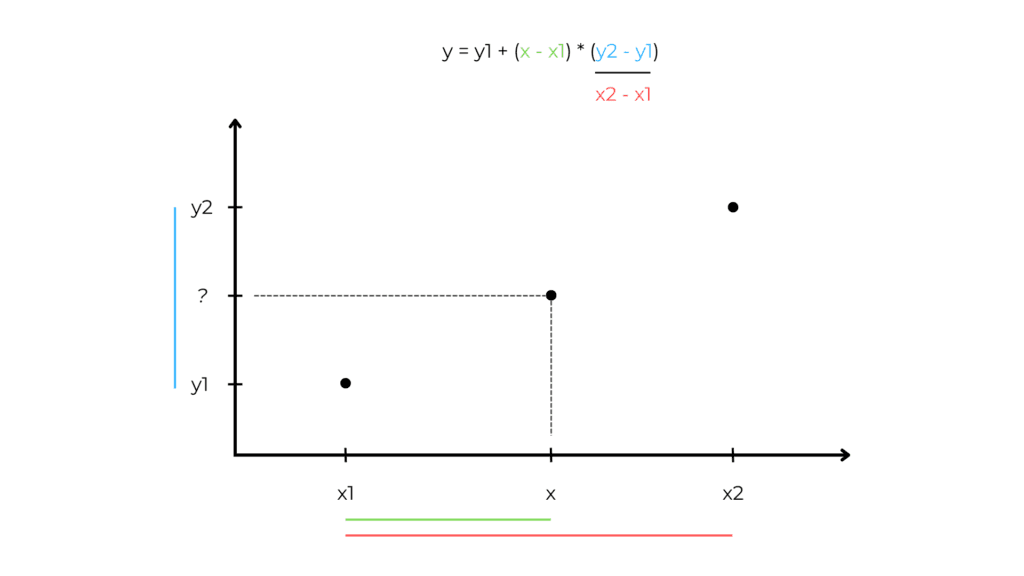
If we have only a feature, the x values are equal to the indexes of the values.
| Cost | Cost |
|---|---|
| 20 | 20 |
| Null | 20 + (26 – 20) / (3 – 1) = 23 |
| 26 | 26 |
| 21 | 21 |
| 24 | 24 |
Python implementation
X = pandas.DataFrame({
    "Time" : [0, 1, 2, 3, 4, 5],
    "Value" : [60, numpy.nan, 80, 50, numpy.nan, 70]
})

new_X = X.interpolate(method = "linear")
When to use these techniques?
We should use these techniques in time series datasets with low and regular variation.
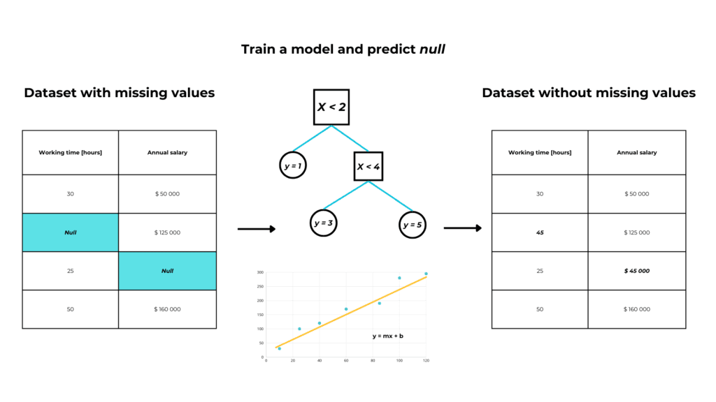
Supervised imputation
We have a feature “α” with missing values and we want to impute them.
So we build a supervised machine-learning model, with:
- y = α, our feature
- X = all the rest of the dataset
If α is numerical, we’ll build a regression model, and if it’s categorical we’ll build a classification model.
Then we use our model to predict the missing values in α.
When to use model imputation?
Since supervised imputation requires time and computational resources, it is most suitable with:
- Datasets with a lot of missing values, especially MNAR values.
- Datasets with a strong correlation between features, or we will build an ineffective model.
Python implementation
from sklearn.experimental import enable_iterative_imputer

from sklearn.impute import IterativeImputer

from sklearn.linear_model import LinearRegression

X = pandas.DataFrame({
    "Salary" : [20000, 45000, 10000, 30000, 35000, 50000],
    "TripCost"  : [numpy.nan, 3000, numpy.nan, 1500, 2500, numpy.nan]
})

imputer = IterativeImputer(estimator=LinearRegression())

new_X = imputer.fit_transform(X)
K-nearest neighbour imputation
To impute the missing values in a feature α, we can build a clustering algorithm like the K-nearest neighbour.
Its input is the observed data from the other features, and it works as follows:
- Create groups of similar data points called clusters
- Assign each row with a missing value in α to a cluster
- Impute missing values in α with the mean α value in the cluster they belong to
Python implementation
from sklearn.impute import KNNImputer

X = pandas.DataFrame({
    "Salary" : [20000, 45000, 10000, 30000, 35000, 50000],
    "TripCost"  : [numpy.nan, 3000, numpy.nan, 1500, 2500, numpy.nan]
})

imputer = KNNImputer()

new_X = imputer.fit_transform(X)
When to use model imputation
Since model imputation requires time and computational resources, it is most suitable with:
- Datasets with a lot of Missing Not at Random Values.
- Datasets with a strong correlation between features, or we will build an ineffective model.