Gradient descent: mathematical background and formula explained

The derivative of a function

Suppose we have a graph representing the population of a village as a function of time.
Let us take two time instants on the x-axis where the population is equal. Now I ask, when did people live better?

Theoretically, there is no difference between x1 and x2, because the population is the same. But if we move the focus from the absolute y value to the variation of y in our instances, we can see that:

• At point x1 the population was increasing. This means that the people were living well.
• At point x2 the population was decreasing. This means that there may had started a famine or a war.

So when we look at data, the change in a value is important. Is this increasing or decreasing, is it changing slowly or quickly?

A derivative can express this information.

What is the derivative of a function?

The derivative of a function is a value that describes the function’s rate of change, i.e. how y varies as x increases.

The derivative of a function is denoted f ‘(x) or df / dx.

Characteristics of a derivative

Now let’s look at some characteristics of a derivative:

• If the derivative is negative, y decreases while x increases.
• If the derivative is positive, y increases while x increases.
• If the derivative is a high number, y is changing rapidly.
• If the derivative is a low number, y is changing slowly.
• If the derivative is a constant, the function is linear, so the relationship between x and y is constant.
• If the derivative is a function, the rate of change of y is not constant and depends on where we are on the abscissa.

Calculate the derivative of a function

Calculating the rate of change of a y with respect to x is intuitive. To an x we add a value such as 1, find the new y, and divide the variation of y by the variation of x, i.e. 1.

This, in a linear graph, corresponds to the angular coefficient of the tangent line.

In fact, the derivative f ‘ (x) at a point x is equivalent to the angular coefficient of the tangent line at x.

But, what is exactly a tangent?

Given a point x on a curve, the tangent line to x is the line through x and a second point infinitely close to it.

Finding the complete formula

The tangent line in a linear relationship graphic is easy to find, it’s just the line with the equation.

However, in dealing with curves, we have to start with 4 points, an initial x, an x with a variation h and their relative outputs. We then have to imagine sliding the second point toward x, decreasing h. It’s when h approaches 0 that we have a tangent.

So, the complete formula to find a derivative is:

• Iim(h -> 0) brings h really close to 0
• f(x + h) – f(x) is the variation of y
• h is the variation of x

Let’s calculate a derivative

The process of finding a derivative is called differentiation.

We have a function f (x) = 4x and we want to calculate the derivative at point 5.

1. Write down the formula.
   
2. Rewrite the function with the attributes and solve
   

Let’s differentiate f (x) = x².

• Write down the formula
  
• Rewrite the function with the attributes and solve
  

In the image we can see how, even though x3 – x2 = x2 – x1, y3 – y2 is way bigger than y2 – y1. That is because if the derivative is a function, the variation depends on the current value of x.

Calculate derivative faster

The partial derivative of a function

A partial derivative of a function with multiple arguments is the derivative with respect to one of the arguments, treating the others as constants.

The vector with all the partial derivatives of a function with multiple arguments is called a gradient, and it is denoted by ∇ f (x).

The gradient descent algorithm

Gradient descent is a parameter optimization algorithm that based on a function’s derivative finds its local minimum.

Before unraveling the mathematical formula to update a parameter using gradient descent, we need to understand the idea behind this algorithm.

How gradient descent works

Problem statement

We have a function f(x) and want to find the optimal value for x that returns in the lowest y.

1. Choose the learning rate and the number of iterations

These hyperparameters are important to choose.

The learning rate determines the size of the steps in updating the parameter. Thanks to the learning rate we reduce the value of the derivative, so that the changes in the parameter are not huge and we do not risk increasing y instead of decreasing it.

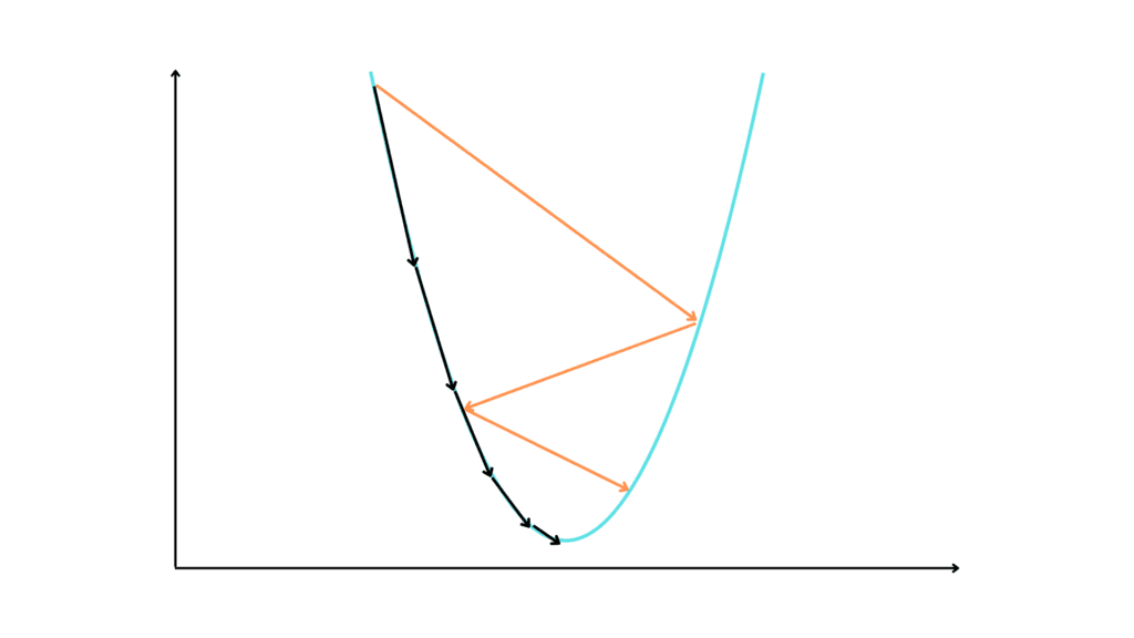
A good learning rate I often use is 0.01.

The number of iterations, or epochs, is the number of times the algorithm updates the value of the parameter.

2. Set the parameter to a random value

The algorithm sets a random initial value of the parameter we want to optimize.

3. Take steps towards the minimum

Then it starts an iteration, where each time it changes the parameter value in order to reach the optimal value where y is at his lowest.

The parameter update formula is this:

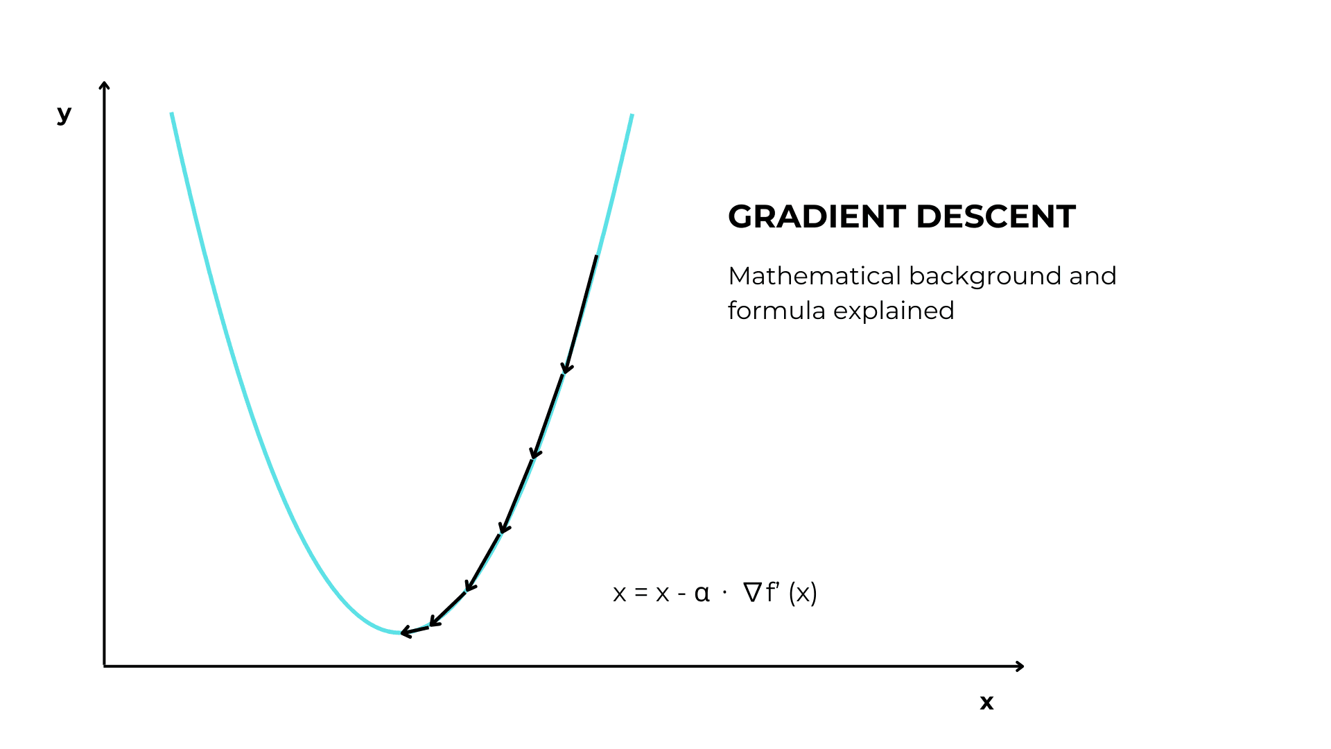
x = x – α ⋅ ∇ f (x)

Where:

• x is the parameter
• α is the learning rate
• ∇ f (x) is the gradient of the function

4. Stop the algorithm

Gradient descent stops when the changes in the parameter are significantly small or it has reached the maximum number of steps.

The idea behind gradient descent

As mentioned above, a derivative expresses the change in y as x increases. This means that if we add the derivative to x the y grows.

If you don’t believe this, look at this example.

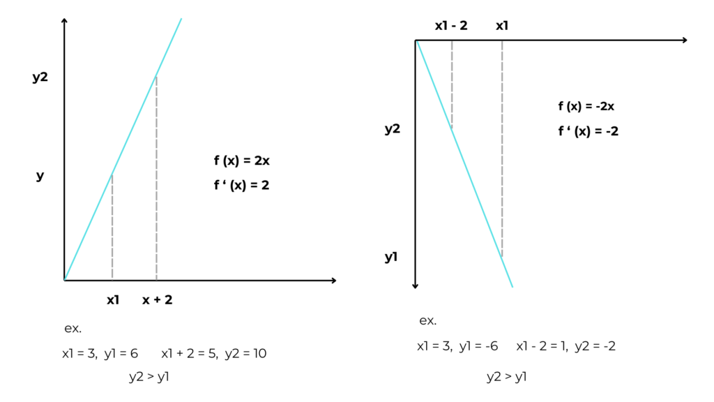
If in adding to x its derivative we increase the value of y, if we subtract from x the derivative we go in the opposite direction, that is, toward the minimum of the function.

The derivative gives us not only the direction in which to move but also the length of the step.

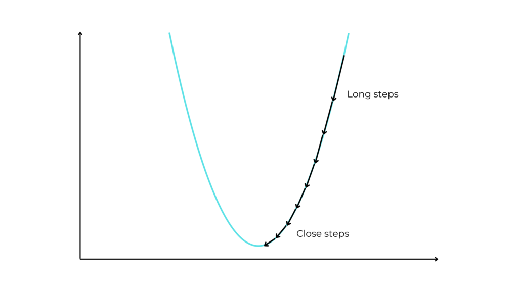
In fact, at more sloping points of the function, the derivative is greater, and consequently, the y has bigger values. So GD takes longer steps because it knows that the lowest value is far. This allows us to reduce training time.

However, it takes shorter steps at flatter points where the minimum may be close and we need to be cautious and precise.

Gradient descent analogy

Imagine being on a mountain at night and wanting to get down to the valley as quickly as possible. You have at your disposal only a flashlight that allows you to see the ground beneath your feet.

To find the lowest point, you look toward the ascent and take steps in the opposite direction, that is, toward the descent.
If the terrain is very steep you take long steps, knowing that you are far from the valley. If the terrain is a little sloping, you take small steps knowing that the lowest point is close.

In this analogy, the mountain is the function and you are the parameter.

Gradient descent limitation

Let’s say we have as input a function like the one in the image.

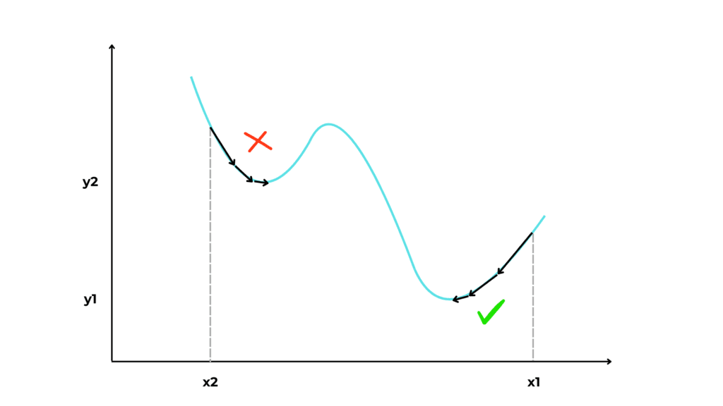
As you can see, if the initial value for x is x1, we successfully reach the lowest point in the function. But if we start from x2, we get to the local minimum in x2 (y2), which is not the global minimum.

Gradient descent types

Batch gradient descent

Batch gradient descent uses all training points at each step to update parameters.

This gives it optimal accuracy but higher computational cost and training time.

Stochastic gradient descent

Stochastic gradient descent uses a random set of training points to update the parameters at each step.

This allows it to have reduced computational cost and training time, but good but not optimal accuracy.

Machine learning algorithms that use gradient descent