Table of Contents
What a decision tree is
A decision tree is a non-parametric supervised machine learning model that predicts outputs by extracting various conditions from the data that an input may or may not meet.
Decision tree structure
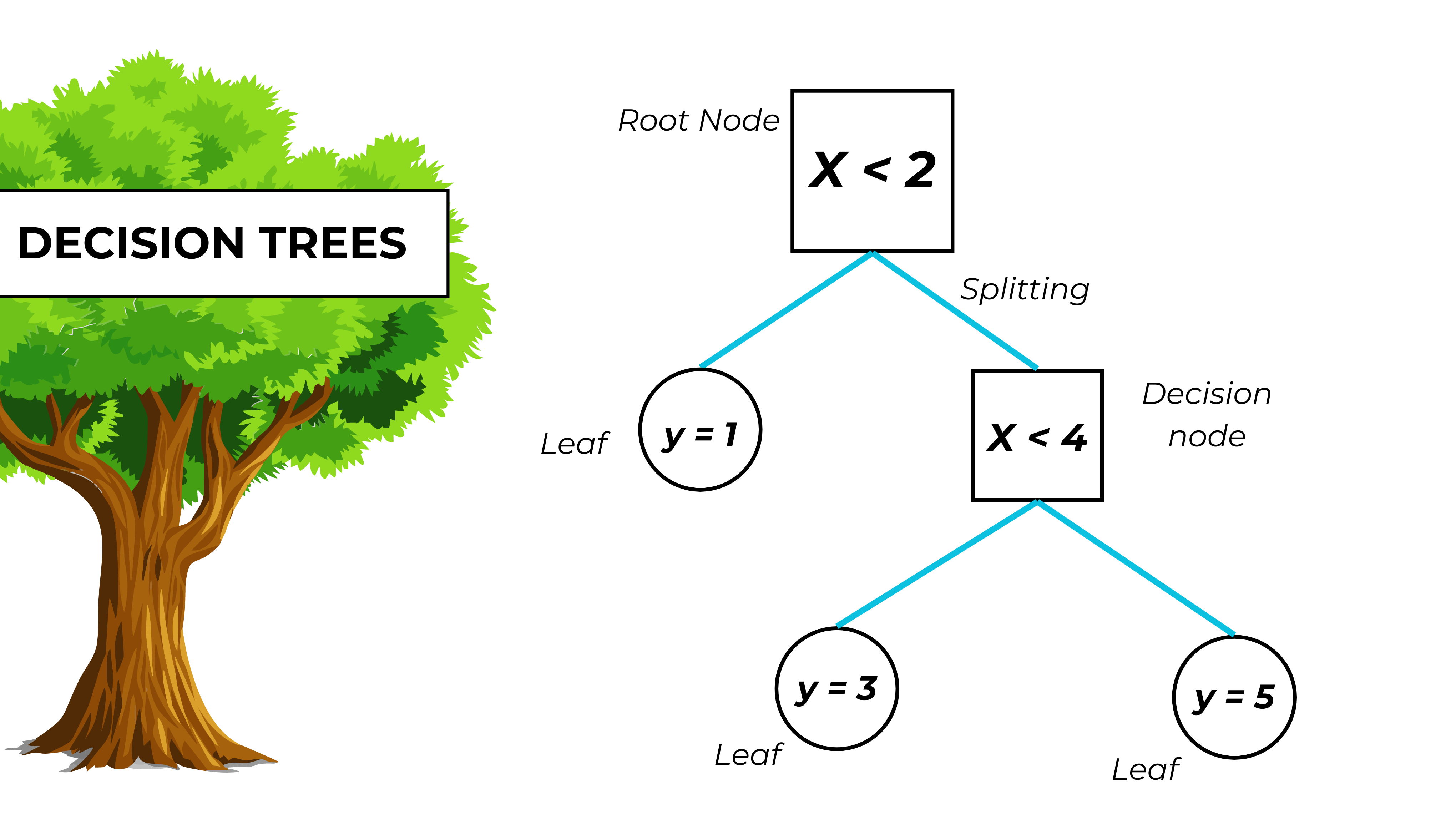
- The root node is the whole input dataset.
- Splitting is dividing an input dataset into subgroups (called nodes).
- Branches are the possible choices or values that the attribute can take. They start from a node; usually, the left branch “is true” and the right one “is false”.
- Leaves (or terminal nodes) represent the final predictions associated with a certain path of decisions.

The CART algorithm: how decision trees work
Problem statement
We have a labeled dataset and want to predict the labels by building a tree-like structure.
1. Extract thresholds and split nodes
For each feature in the dataset, the algorithm iterates through each value and uses it as a threshold to split the dataset into two nodes.
If the current feature is numerical, the algorithm assigns data points to the nodes whether their feature value is smaller or equal to the threshold.
If the current feature is categorical, the algorithm assigns data points to the nodes whether their feature value is equal to the threshold.
2. Choose the optimal thresholds
For each threshold, the algorithm calculates the impurity of its sub-nodes.
The impurity is a parameter that expresses the similarity of the outputs of a node.
Why is impurity important?
Impurity is used to measure the quality of a split.
If the impurity is low => the samples in the node are similar => the threshold is good because it highlights a characteristic that these data points share.
So when we are trying to predict an unseen value, and we see that it has this characteristic, it makes sense to predict an output similar to the other samples in the node.
2.1 Impurity in classification
In classification, impurity is calculated using the Gini impurity parameter, which expresses the homogeneity of the samples in a node.
Where:
- N = total number of samples in the node.
- Nn = total number of samples in the node of class n.
Curiosity: why do we square the probabilities?
We square the probabilities because otherwise, the total sum would always equal 1.
To understand, the lower the Giny Impurity of a node, the more examples in that node are of the same class.

2.2 Impurity in regression
The impurity of a node in a regression problem is equal to the mean squared residual.
For each data point in the node, the square residual is:
Where:
- y = output of the data point,
- mean y = average value of all the node outputs.
Choose the threshold
This is the formula called weighted impurity:
Where:
- N is the number of data points in a node.
The threshold with the lowest weighted impurity is chosen to split the dataset.
3. Stop the tree from growing
The splitting process of a node ends when its impurity is minimal, or when its number of data points in the value of the hyperparameter min_samples_leaf. At this point, the node becomes a leaf.
The learning process stops entirely (the tree stops growing) when the value of the max_depth or max_leaves_num is reached.
4. Predict outputs
For each input, the model follows a decision path. The prediction value is the average output of the leave in which the input falls.
Model main hyperparameters
These are the model’s main hyperparameters taken from the scikit-learn documentation.
- max_depth: The maximum depth of the tree. If None, then nodes are expanded until all leaves are pure or until all leaves contain less than min_samples_split samples.
- max_leaves_num: The maximum number of leaves in the model.
- min_samples_split: The minimum number of samples required to split an internal node.
- min_samples_leaf: The minimum number of samples required to be at a leaf node.
Decision tree advantages and disadvantages
Advantages
- Simple to understand and to interpret. Trees can be visualized.
- Requires little feature engineering. Other techniques often require data normalization, dummy variables need to be created and blank values need to be removed. Some tree and algorithm combinations support missing values.
- Able to handle both numerical and categorical data.
- Able to handle multi-output problems.
- Uses a white box model. If a given situation is observable in a model, the explanation for the condition is easily explained by boolean logic (true or false). By contrast, results may be more difficult to interpret in a black box model (e.g., in an artificial neural network).
- Possible to validate a model using statistical tests. That makes it possible to account for the reliability of the model.
- Decision trees make it easy to evaluate feature importance, or contribution, to the model.
There are a few ways to evaluate feature importance, like the gini importance measure of a feature, which equals the average information gain of nodes related to that feature.
Disadvantages
- Decision-tree learners can create over-complex trees that do not generalize the data well. This is called overfitting. Mechanisms such as pruning, setting the minimum number of samples required at a leaf node or setting the maximum depth of the tree are necessary to avoid this problem.
- Decision trees can be oversensitive and unstable because small variations in the data might result in a completely different tree being generated. This problem is mitigated by using decision trees within an ensemble (such as the random forest model or XGBoost).
- Decision tree learners create biased trees if some classes dominate. It is therefore recommended to balance the dataset before fitting with the decision tree.
These aspects are taken from the general scikit-learn documentation about decision trees.
Programming a decision tree
From now you are going to learn how to build a decision tree model in Python using the scikit-learn library.
1. Import necessary libraries
The libraries used in this project are:
- Pandas for handling input and output data.
- Math for the square root function.
- Sklearn for importing the decision tree algorithm and the validation metric.
- Matplotlib for visualizing the model structure.
import pandas

from sklearn.model_selection import train_test_split

from sklearn import tree

from sklearn.tree import DecisionTreeRegressor

from sklearn.metrics import mean_squared_error

from matplotlib import pyplot as plt
2. Upload the dataset
#upload the dataset

dataset = pandas.read_csv( "C:\\...\\realestate_dataset.csv")
The data used to train this model look something like this:
| Rooms | Building area | Year Built | … | Sale price | |
| 1 | 8 | 150 | 1987 | 650 000 | |
| 2 | 5 | 95 | 2015 | 300 000 | |
| 3 | 6 | 105 | 1967 | 130 000 | |
| 4 | 4 | 75 | 2001 | 75 000 |
The dataset I used is a real estate dataset that reports the sales values of properties with their respective building characteristics.
3. Select input and output features and split the data
#define the features and the label

input_variables = ['LotArea', 'OverallQual', 'YearBuilt', '1stFlrSF', '2ndFlrSF', 'FullBath', 'BedroomAbvGr', 'KitchenAbvGr', 'TotRmsAbvGrd']

X = dataset[input_variables]

y = dataset[["SalePrice"]]

train_X, val_X, train_y, val_y = train_test_split(X, y) #split the data into training and testing data
4. Train and validate the model
#load and train the model

model = DecisionTreeRegressor(max_depth=6)

model.fit(train_X, train_y)


#evaluate model's performance using the root mean squared error performance

RMSE = math.sqrt(
    mean_squared_error(val_y, model.predict(val_X))
)

print(RMSE)
Wow! The root mean squared error of our model is 41 034. It means that on average, the real value differs by $ 41 034 from the predicted price for each prediction. For guessing house prices this isn’t a bad result.
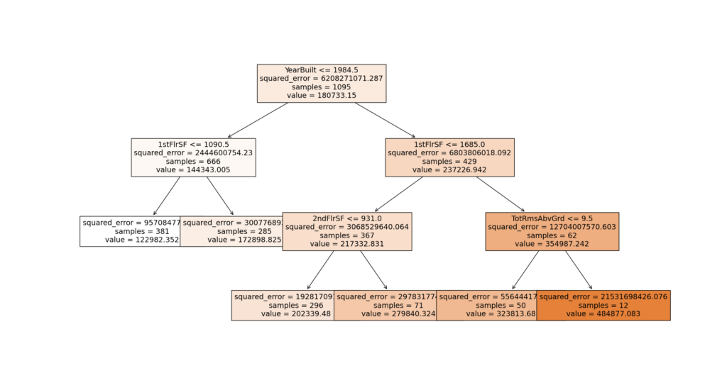
5. Visualize the model
#show model structure textual and visual representation

text_representation = tree.export_text(model)


pyplot.figure(figsize=(25,20))

tree.plot_tree(model, feature_names=input_variables, filled=True)

pyplot.show()
Decision tree full code
import pandas

import math

from sklearn import tree

from sklearn.tree import DecisionTreeRegressor

from sklearn.metrics import mean_squared_error

from sklearn.model_selection import train_test_split

from matplotlib import pyplot


#upload the dataset

dataset = pandas.read_csv( "C:\\...\\realestate_dataset.csv")


#define the features and the label

input_variables = ['LotArea', 'OverallQual', 'YearBuilt', '1stFlrSF', '2ndFlrSF', 'FullBath', 'BedroomAbvGr', 'KitchenAbvGr', 'TotRmsAbvGrd']

X = dataset[input_variables]

y = dataset[["SalePrice"]]

train_X, val_X, train_y, val_y = train_test_split(X, y) #split the data into training and testing data


#load and train the model

model = DecisionTreeRegressor(max_depth=6)

model.fit(train_X, train_y)


#evaluate model's performance using the root mean squared error performance

RMSE = math.sqrt(
    mean_squared_error(val_y, model.predict(val_X))
)

print(RMSE)


#show model structure textual and visual representation

text_representation = tree.export_text(model)
print(text_representation)


plt.figure(figsize=(25,20))

tree.plot_tree(model, feature_names=input_variables, filled=True)

plt.show()