Table of Contents
What is a random forest?
A random forest is a bagging machine-learning model that combines the output of numerous decision trees to make predictions.
Random forest training
As said before, the random forest algorithm is just the bagging (bootstrap aggregation) algorithm, an ensemble training technique, that trains numerous decision trees.
I’ve written an article about bagging and I suggest you read it, but it’s not necessary because everything you need to know about random forests is explained below.
1. Bootstrapping
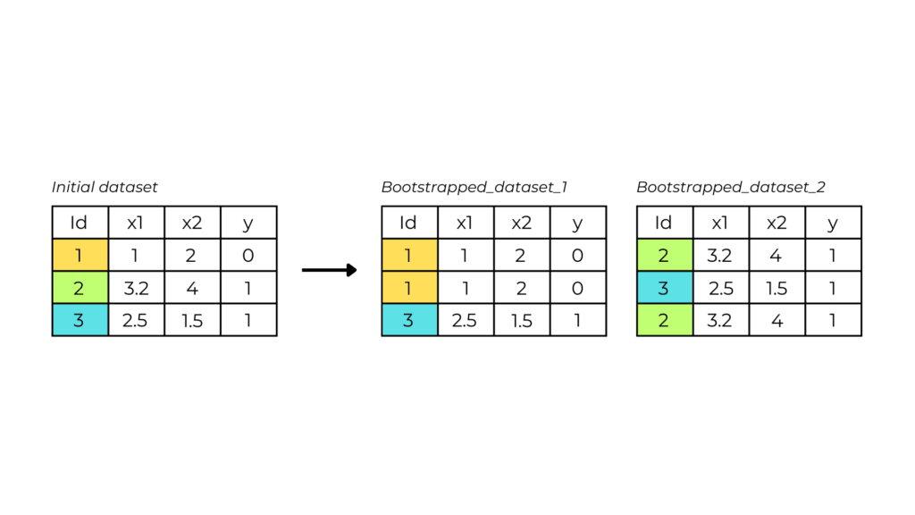
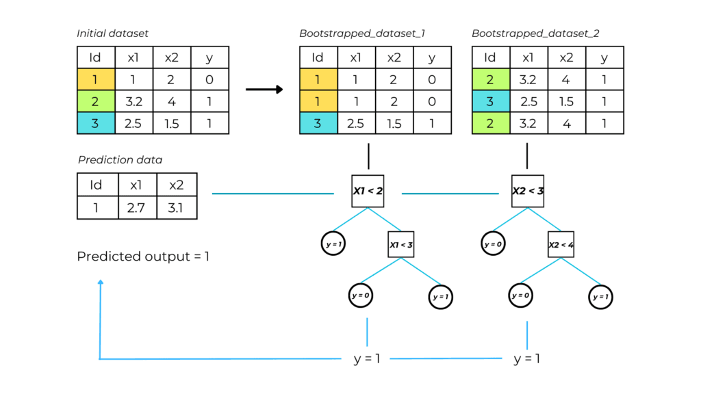
Bootstrapping is creating many copies of the original dataset by randomly selecting observations.
Let N be the length of dataset X. Bootstrapping generates datasets of size N, with each slot filled by a randomly selected observation from X.
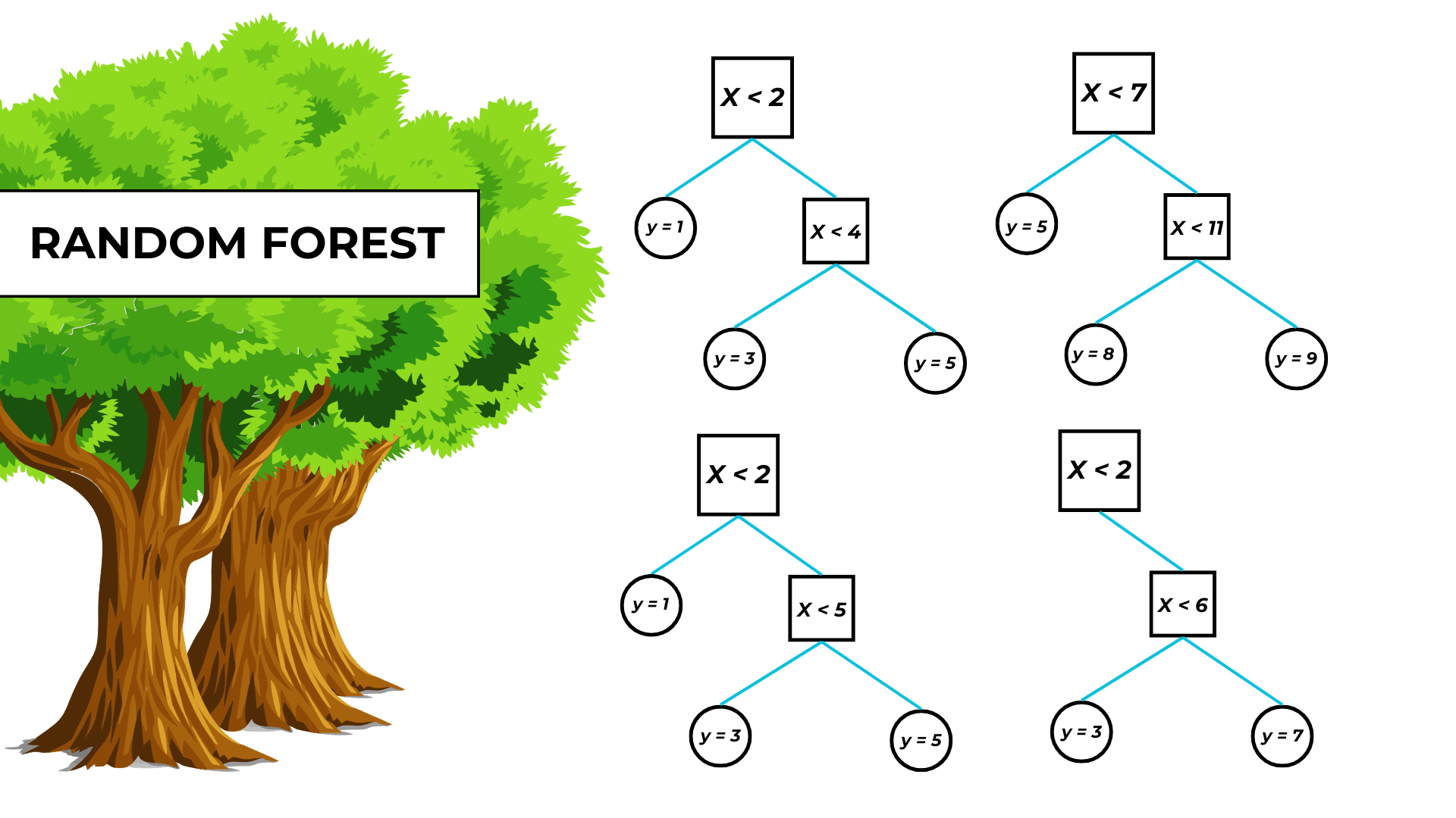
2. Tree construction
A decision tree is built and independently trained on every new bootstrapped dataset.
3. Output prediction through aggregation
The random forest output is the mean value of all the trees’ predictions.
In machine learning, combining results from multiple models is called aggregation.
Why is randomness in a random forest so important?
Bootstrapping is vital in a random forest model because it ensures that every tree is trained on different data. This helps our model be less sensitive and dependent on the original training data, therefore improving the overfitting problem of single decision trees.
They are also useful because they prevent trees from being too similar. After all, with the same features, they would probably share similar decision nodes.
Random forest main hyperparameters
These are the main hyperparameters taken from the scikit-learn documentation about parameters. You can check the parameters for the decision trees, which also apply to this model, in their article.
- n_estimators: the number of trees in the forest.
- max_depth: the maximum depth of the tree. If None, then nodes are expanded until all leaves are pure or until all leaves contain less than min_samples_split samples.
- max_leaves_num: the maximum number of leaves in the model.
- min_samples_split: the minimum number of samples required to split an internal node.
- min_samples_leaf: the minimum number of samples required to be at a leaf node.
Decision tree advantages and disadvantages
Advantages
A random forest model maintains the benefits of a decision tree, in addition to the things below.
- As already mentioned, decision trees sometimes can be oversensitive and run the risk of overfitting. However, a random forest model won’t overfit, thanks to the number of trees and feature bagging.
- Feature bagging also makes the random forest classifier an effective tool for estimating missing values as it maintains accuracy when a portion of the data is missing.
To be clear missing values present in a specific row will not affect pieces of the database that do not contain it. - It is possible to use parallel processing to distribute the training and prediction process among processors, thus decreasing time. The number of processors is adjustable with the n_jobs parameter seen earlier.
Disadvantages
- Since random forest algorithms can handle large data sets, they can provide more accurate predictions but can be slow to process data and can require more resources
- It is difficult to fully visualize, analyze, and interpret the model as it is composed of numerous trees.
Programming a random forest model
1. Import necessary libraries
The libraries used in this project are:
- Pandas for handling input and output data.
- Math for the square root function.
- Sklearn for importing the random forest algorithm and the validation metric.
- Matplotlib for visualizing the model structure.
import pandas as pd

import joblib

import sklearn

from sklearn import tree

from sklearn.tree import DecisionTreeRegressor

from sklearn.metrics import mean_absolute_error

from sklearn.model_selection import train_test_split

from matplotlib import pyplot as plt
2. Upload the dataset
#upload the dataset

dataset = pd.read_csv("C:\\...\\realestate_dataset.csv")
The data used to train this model look something like this:
| Rooms | Building area | Year Built | … | Sale price | |
| 1 | 8 | 150 | 1987 | 650 000 | |
| 2 | 5 | 95 | 2015 | 300 000 | |
| 3 | 6 | 105 | 1967 | 130 000 | |
| 4 | 4 | 75 | 2001 | 75 000 |
The dataset I used is a real estate dataset that reports the sales values of properties with their respective building characteristics.
3. Select input and output features
#define the features and the label

input_variables = ['LotArea', 'OverallQual', 'YearBuilt', '1stFlrSF', '2ndFlrSF', 'FullBath', 'BedroomAbvGr', 'KitchenAbvGr', 'TotRmsAbvGrd']

X = dataset[input_variables]

y = dataset[["SalePrice"]]

train_X, val_X, train_y, val_y = train_test_split(X, y) #split the data into training and testing data
4. Train and validate the model
#load and train the model

model = RandomForestRegressor(max_depth=6)

model.fit(train_X, train_y)


#evaluate model's performance using the root mean squared error performance

RMSE = math.sqrt(
    mean_squared_error(val_y, model.predict(val_X))
)

print(RMSE)
Wow! The root mean squared error of our model is 41 034. It means that on average, the real value differs by $ 41 034 from the predicted price for each prediction. For guessing house prices this isn’t a bad result.
5. Visualize the model structure
#show model's trees individual structure textual and visual representation through indexing

plt.figure(figsize=(25,20))
tree.plot_tree(model.estimators_[0],
                   filled = True)
plt.show()
Random forest full code
import pandas as pd

import math

from sklearn import tree

from sklearn.ensemble import RandomForestRegressor

from sklearn.metrics import mean_squared_error

from sklearn.model_selection import train_test_split

from matplotlib import pyplot as plt


#upload the dataset

dataset = pd.read_csv("C:\\...\\realestate_dataset.csv")


#define the input and the output

input_variables = ['LotArea', 'OverallQual', 'YearBuilt', '1stFlrSF', '2ndFlrSF', 'FullBath', 'BedroomAbvGr', 'KitchenAbvGr', 'TotRmsAbvGrd']

X = dataset[input_variables]

y = dataset[["SalePrice"]]

train_X, val_X, train_y, val_y = train_test_split(X, y, random_state = 0) #split the data into training and testing data


#load and train the model

model = RandomForestRegressor(max_depth=4, n_estimators=100)

model.fit(train_X, train_y.values.ravel())


#evaluate model's performance using the root mean squared error performance

RMSE = math.sqrt(
    mean_squared_error(val_y, model.predict(val_X))
)

print(RMSE)


#show model's trees individual representation

plt.figure(figsize=(25,20))
tree.plot_tree(model.estimators_[0])
plt.show()