Table of Contents
What is bagging?
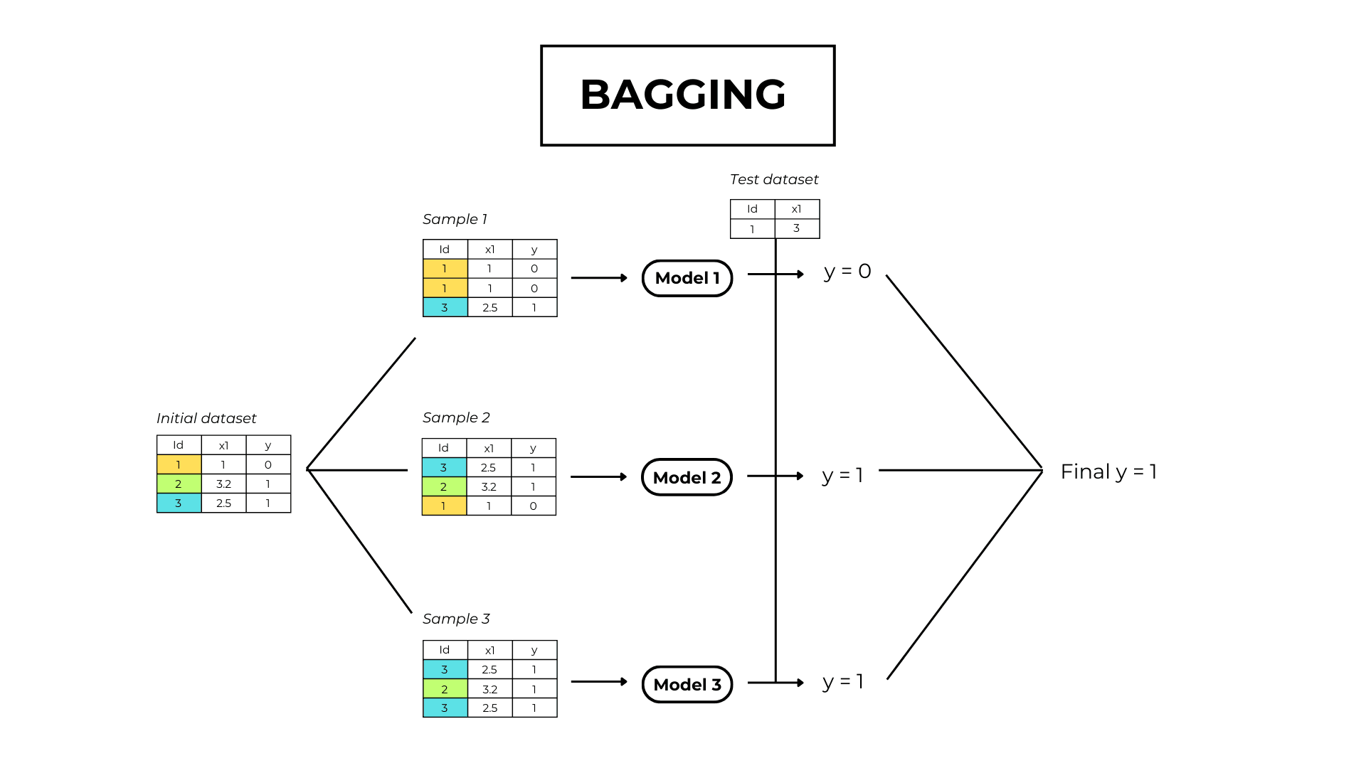
Bagging is a parallel ensemble learning technique that trains multiple weak models on different datasets and averages their predictions.
The bagging algorithm
Problem statement
We have a dataset and want to build an ensemble model to make predictions.
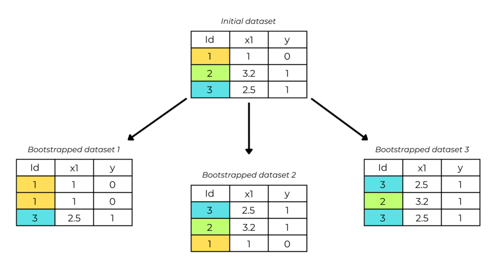
1. Bootstrapping
In the bootstrapping phase, we create many copies of the original dataset by randomly selecting observations.
Let N be the length of dataset X. Bootstrapping generates datasets of size N, with each slot filled by a randomly selected observation from X.
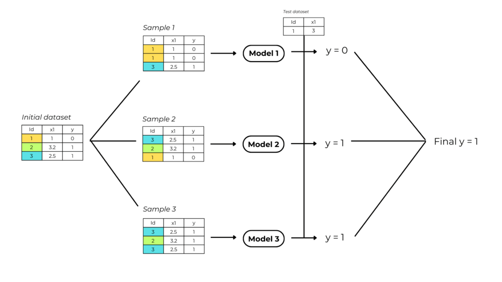
2. Model training
We train a simple model (“weak learner”) for each bootstrapped dataset we’ve created.
3. Make predictions with aggregation
The model output is the mean value of all the weak learner’s predictions.
In machine learning, combining results from multiple models is called aggregation.
Why is it called bagging?
The word bagging comes from two machine learning techniques bootstrapping and aggregating.
Bagging benefits. Why do we use it?
Using an ensemble bagging model has many benefits.
Reduced variance
Bootstrapping is vital in a bagging ensemble because it ensures that every weak learner is trained on different data. This helps our model be less sensitive and dependent on the original training data, reducing variance and overfitting change.
Diverse models
Using different data also prevents the algorithm from training weak learners that otherwise would be too similar.
Computationally efficient
Since weak learners are trained independently in bagging, we can run the training processes in parallel and save time and energy.
Bagging vs Gradient boosting vs AdaBoost
| Bagging | Gradient boosting | AdaBoost | |
|---|---|---|---|
| Dataset | Bootstrapped samples | Default | Weighted observations |
| Single tree structure | Default | Default | A stump (1 split) |
| Target feature | Output feature | Pseudo residuals | Output feature |
| Training | Parallel | Sequential | Sequential |
| Contribution scaling | None | Constant | Depends on each model’s accuracy |
| Main focus | Reduce variance | Reduce bias | Reduce bias |
Bagging in Python
From now on, you will learn how to build a model using bagging in Python using the scikit-learn library.
1. Import necessary libraries
import pandas as pd

import math

from sklearn.model_selection import train_test_split

from sklearn.linear_model import LinearRegression

from sklearn.ensemble import BaggingRegressor

from sklearn.metrics import mean_squared_error

from matplotlib import pyplot as plt
The libraries used in this project are:
- Pandas for handling input and output data.
- Math for the square root function.
- Sklearn for importing the decision tree algorithm, validation parameter, and preprocessing techniques.
- Matplotlib for visualizing the model structure.
2. Upload the dataset
#upload the dataset
file_path = "C:\\...\\melb_data.csv" #real estate data with house prices and input details

dataset = pd.read_csv(file_path)
The data used to train this model look something like this:
| Rooms | Building area | Year Built | … | Sale price | |
| 1 | 8 | 150 | 1987 | 650 000 | |
| 2 | 5 | 95 | 2015 | 300 000 | |
| 3 | 6 | 105 | 1967 | 130 000 | |
| 4 | 4 | 75 | 2001 | 75 000 |
The dataset I used is a real estate dataset that reports the sales values of properties with their respective building characteristics.
3. Select input and output features and split the data
#define the features and the label

X = dataset[["LotArea"]]

y = dataset[["SalePrice"]]

train_X, val_X, train_y, val_y = train_test_split(X, y) #split the data into training and testing data
4. Train and evaluate the model
#load and train the model

model = BaggingRegressor(LinearRegression(), n_estimators = 300) # n_estimators is the number of weak learners we want to build

model.fit(train_X, train_y)

print(math.sqrt(mean_squared_error(val_y, model.predict(val_X)))) #evaluate it's performance
The root mean squared error of our model is 70 075. This means that on average, our model is off $ 70 075 for every prediction.
It’s a relatively high value, but we must consider that this dataset is too complex and imbalanced for linear regression
Bagging in Python full code
import pandas as pd

import math

from matplotlib import pyplot as plt

from sklearn.model_selection import train_test_split

from sklearn.linear_model import LinearRegression

from sklearn.ensemble import BaggingRegressor

from sklearn.metrics import mean_squared_error


#upload the dataset

file_path = "C:\\Users\\ciaos\\Documents\\blog\\posts\\blog post information\\Linear regression\\realestate_dataset.csv"

dataset = pd.read_csv(file_path)

#define the features and the label

X = dataset[["LotArea"]]

y = dataset[["SalePrice"]]

train_X, val_X, train_y, val_y = train_test_split(X, y) #split the data into training and testing data


#load and train the model

model = BaggingRegressor(LinearRegression(), n_estimators=300)

model.fit(train_X, train_y)

print(math.sqrt(mean_squared_error(val_y, model.predict(val_X)))) #evaluate it's performance