Table of Contents
What linear regression is
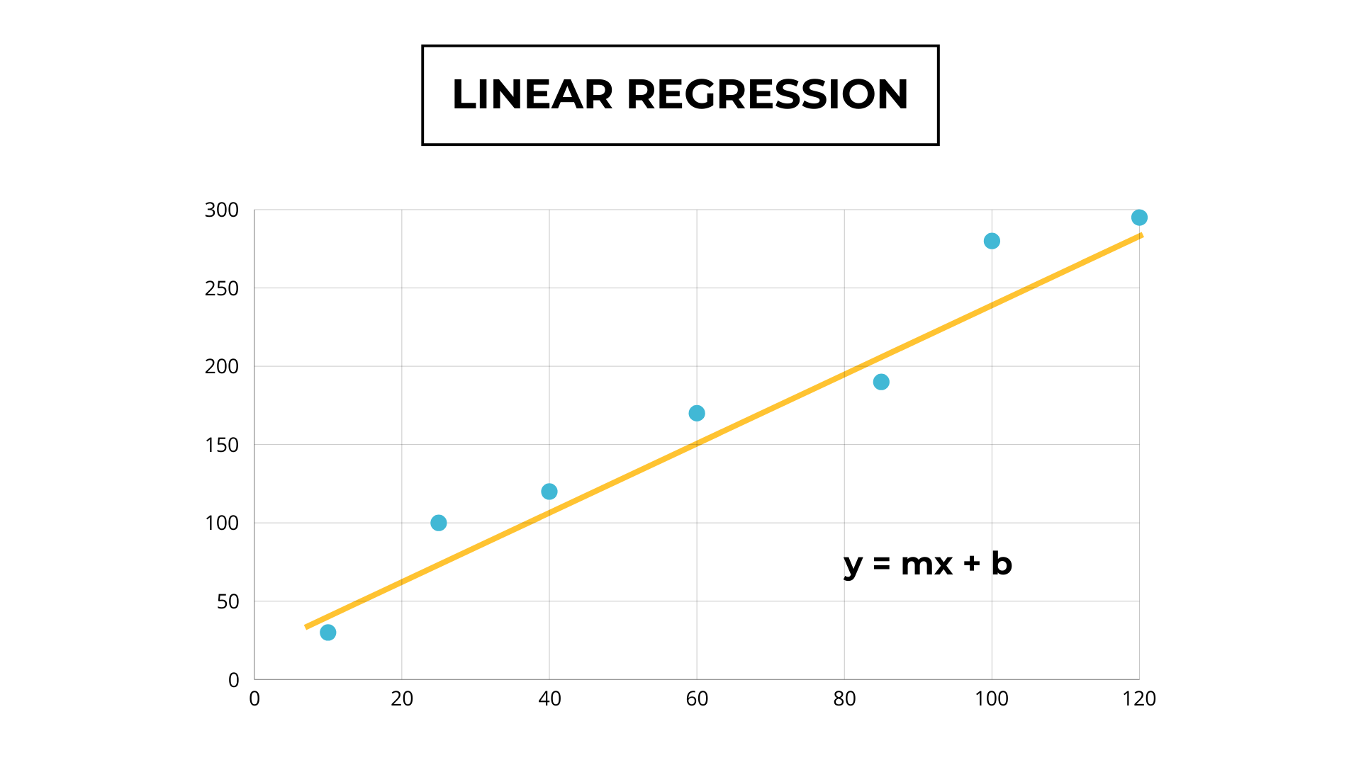
Linear regression is a supervised machine-learning algorithm that fits a straight line to the input data to represent the relationship between x and y.
Linear regression structure
Suppose we have a dataset that contains two columns, one with the area in m2 of some houses and the other with their prices.
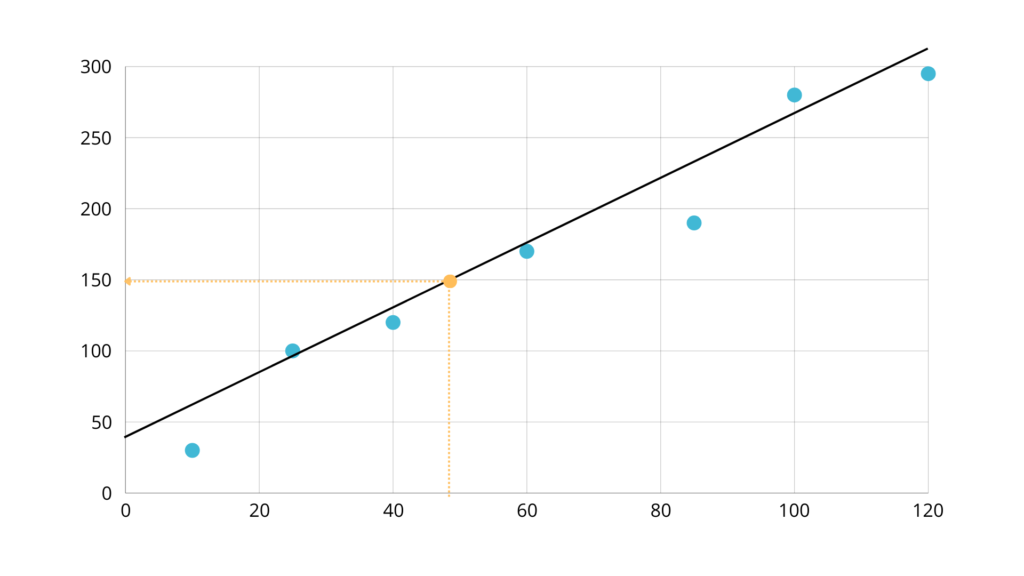
We can plot the data on a graph, which would look something like this:
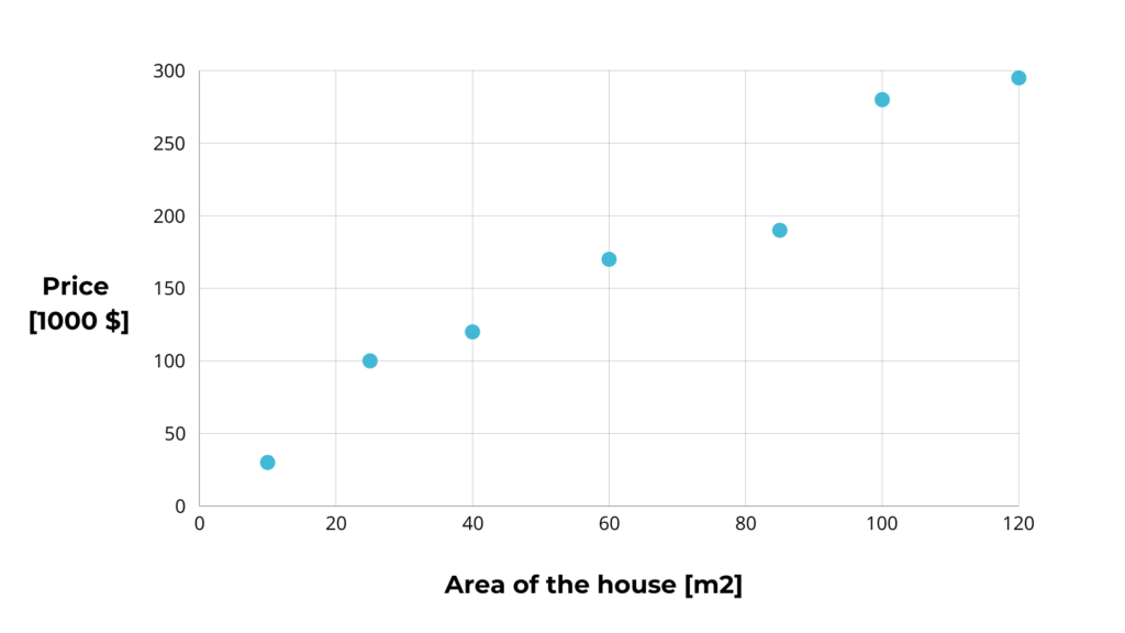
We are investors and want to predict the price of a house based on its area. This means that the column with the area is the input column X. The price is the output column y.
The algorithm aims to find a line that best represents the relationship between X and y. Extending a point from the x-axis makes it possible to determine its value on the y-axis, which is the height where it intersects with the line.
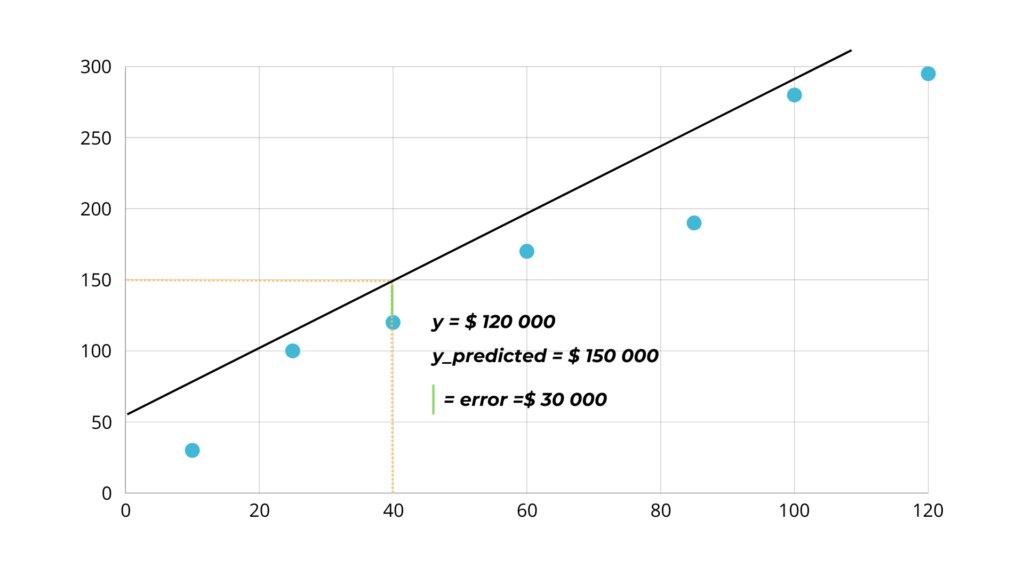
But for the predictions to be accurate the line has to pass through the points, because otherwise, as in the example below, the difference between the y and the predicted y is $30,000.
This means that the error of our calculations is equal to the distance between the point and the line.
The task of the algorithm is then to move the line so that it is as close as possible to all the data points by adjusting two parameters:
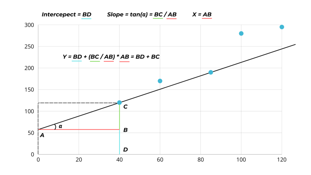
- The slope is the tangent of the angle of the line with the x-axis.
Mathematically, it tells us how much y changes when x changes 1. - The intercept, is the point where the line intersects with the y-axis.
So the mathematical formula for y is:
How linear regression works
Problem statement
We have a dataset with a numerical label (regression problem). We want to fit a straight line as close to all the data points to represent the relationship between x and y.
1. Initialize the intercept and slope
Initially, the algorithm set both our parameters, the intercept, and the slope, to 0.
2. Fit the line with gradient descent
To fit the line it uses gradient descent, a powerful algorithm that optimizes parameter value to minimize a given function.
The function in this case we want to optimize is the squared distance between the data points and our line, i.e. the square residuals.
Where:
- N is the number of data points,
- y is the real output value,
- x is the input value.
2.1 Calculate the sum of gradients
The algorithm calculates the partial derivative of E with respect to w and b at each data point.
And then it sums them up.
2.2 Update the parameters
To update the parameters, the algorithm subtracts from the initial value the derivative multiplied by a small learning rate (α).
The algorithm updates parameters until the change is minimal or a maximum iteration is reached.
3. Predict outputs
To predict an output we just have to plug it in the formula y = b + wx, where b and w are the constants we have just found.
Linear regression types
Simple linear regression
Describes the relationship between one independent and one dependent variable.
Multiple linear regression
Describes the relationship between multiple independent variables and one dependent variable.
From simple linear regression, the structure formula changes slightly.
Now for every new feature, we have a new slope.
Linear regression advantages and disadvantages
Linear regression advantages
- Since linear regression is a simple model, it is computationally cheap, simple, and fast to train.
- Linear regression is perfect for representing linear relationships between data.
- Linear regression is a white box model. This means that his internal work and decision-making process is clear. That’s because we know the exact value of w and b
Linear regression disadvantages
- Linear regression is very sensible to outliers. Outliers are rare data that differ significantly from the mean values of the other observations.
- Linear regression can’t represent non-linear relationships between data.
When to use linear regression?
I think it’s always a good thing to try a linear regression model as a baseline.
Linear regression is especially good when:
- Our target feature Is continuous (regression problem).
- The relationship between X and y is somehow linear.
- We don’t want to spend much time training the model
Linear regression in Python
1. Import necessary libraries
import pandas as pd

import math

from sklearn.model_selection import train_test_split

from sklearn.linear_model import LinearRegression

from sklearn.metrics import mean_squared_error

from matplotlib import pyplot as plt
The libraries used in this project are:
- Pandas for handling input and output data.
- Math for the square root function.
- Sklearn for importing the decision tree algorithm, validation parameter, and preprocessing techniques.
- Matplotlib for visualizing the model structure.
2. Upload the dataset
#upload the dataset
file_path = "C:\\...\\melb_data.csv" #real estate data with house prices and input details

dataset = pd.read_csv(file_path)
The data used to train this model look something like this:
| Rooms | Building area | Year Built | … | Sale price | |
| 1 | 8 | 150 | 1987 | 650 000 | |
| 2 | 5 | 95 | 2015 | 300 000 | |
| 3 | 6 | 105 | 1967 | 130 000 | |
| 4 | 4 | 75 | 2001 | 75 000 |
The dataset I used is a real estate dataset that reports the sales values of properties with their respective building characteristics.
3. Select input and output features and split the data
#define the features and the label

X = dataset[["LotArea"]]

y = dataset[["SalePrice"]]

train_X, val_X, train_y, val_y = train_test_split(X, y) #split the data into training and testing data
4. Train and evaluate the model
#load and train the model

model = LinearRegression()

model.fit(train_X, train_y)

print(math.sqrt(mean_squared_error(val_y, model.predict(val_X)))) #evaluate it's performance
The root mean squared error of our model is 78 121. This means that on average, our model is off $ 78 121 for every prediction.
It’s a relatively high value, but we must consider that this dataset is too complex and imbalanced for linear regression.
5. Print the 2 parameters
# display the 2 parameters

print(float(model.intercept_), float(model.coef_[0]))
The model slope is 2.03 and the model intercept is 159264.
This means that to predict, this model just takes an input x, multiplies it by 2.03, and adds 159 264.
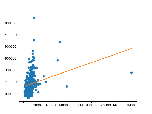
6. Visualize the model
#plot the model and the dataset on a graph

plt.plot(val_X["LotArea"], val_y["SalePrice"], "o", val_X["LotArea"], [float(model.intercept_) + x * float(model.coef_[0]) for x in val_X["LotArea"]])

plt.show()
This is the result:
Linear regression full code
import pandas as pd

import math

from matplotlib import pyplot as plt

from sklearn.model_selection import train_test_split

from sklearn.linear_model import LinearRegression

from sklearn.metrics import mean_squared_error


#upload the dataset

file_path = "C:\\Users\\ciaos\\Documents\\blog\\posts\\blog post information\\Linear regression\\realestate_dataset.csv"

dataset = pd.read_csv(file_path)

#define the features and the label

X = dataset[["LotArea"]]

y = dataset[["SalePrice"]]

train_X, val_X, train_y, val_y = train_test_split(X, y, random_state = 0) #split the data into training and testing data


#load and train the model

model = LinearRegression()

model.fit(train_X, train_y)

print(math.sqrt(mean_squared_error(val_y, model.predict(val_X)))) #evaluate it's performance


# display the 2 parameters

print(float(model.intercept_), float(model.coef_[0]))


#plot the model and the dataset on a graph

plt.plot(val_X["LotArea"], val_y["SalePrice"], "o", val_X["LotArea"], [float(model.intercept_) + x * float(model.coef_[0]) for x in val_X["LotArea"]])

plt.show()