Table of Contents
Disclaimer
The gradient descent algorithm is based on the concept of the derivative of a function. Check this article before continuing.
The gradient descent algorithm
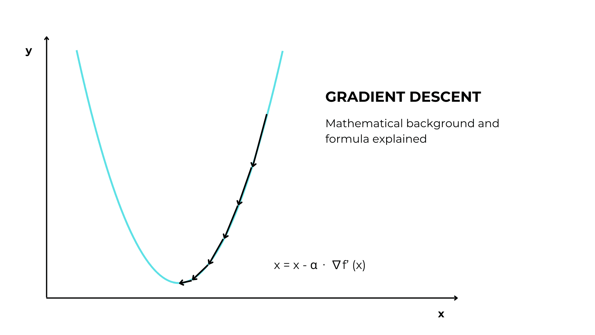
Gradient descent is a parameter optimization algorithm. Given an input function f(x), it finds the x value where y is the lowest.
Problem statement
We have a function f(x) and want to find the optimal value for x that returns in the lowest y.
1. Choose the learning rate and the number of iterations
These hyperparameters are important to choose.
The learning rate determines the size of the steps in updating the parameter. Thanks to the learning rate we reduce the value of the derivative, so that the changes in the parameter are not huge and we do not risk increasing y instead of decreasing it.
A good learning rate I often use is 0.01.
The number of iterations, or epochs, is the number of times the algorithm updates the value of the parameter.
2. Set the parameter to a random value
The algorithm sets a random initial value of the parameter we want to optimize.
3. Take steps towards the minimum
Then it starts an iteration, where each time it changes the parameter value in order to reach the optimal value where y is at his lowest.
The parameter update formula is this:
x = x – α ⋅ ∇ f (x)
Where:
- x is the parameter
- α is the learning rate
- ∇ f (x) is the gradient of the function
4. Stop the algorithm
Gradient descent stops when the changes in the parameter are significantly small or it has reached the maximum number of steps.
The idea behind gradient descent
The direction we want to move towards
As mentioned above, a derivative expresses the change in y as x increases. This means that if we add the derivative to x the y grows.
If you don’t believe this, look at this example.
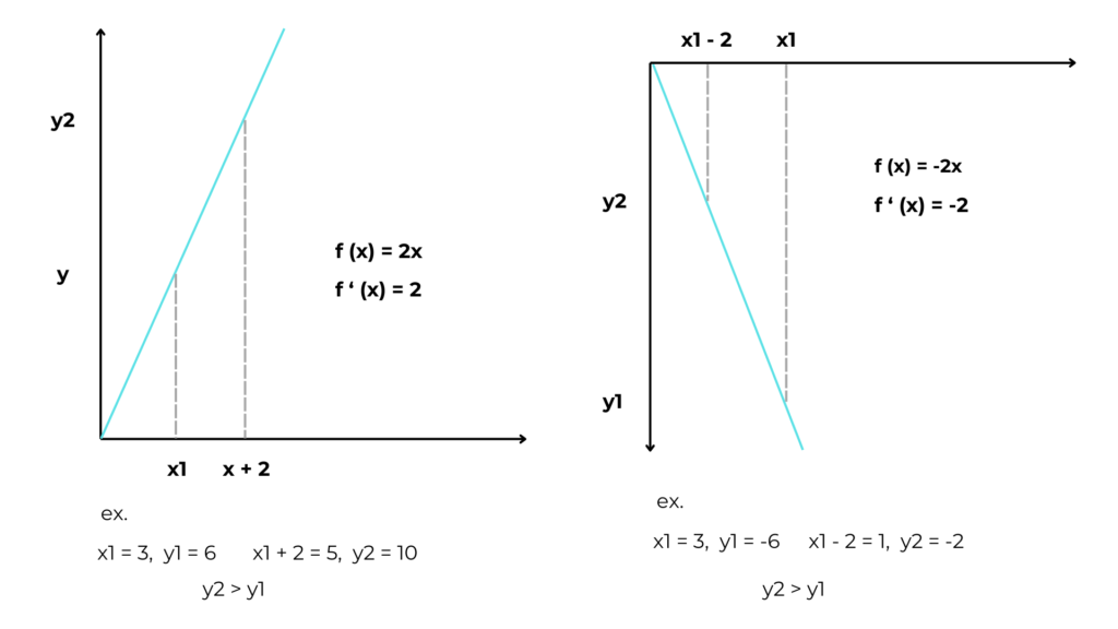
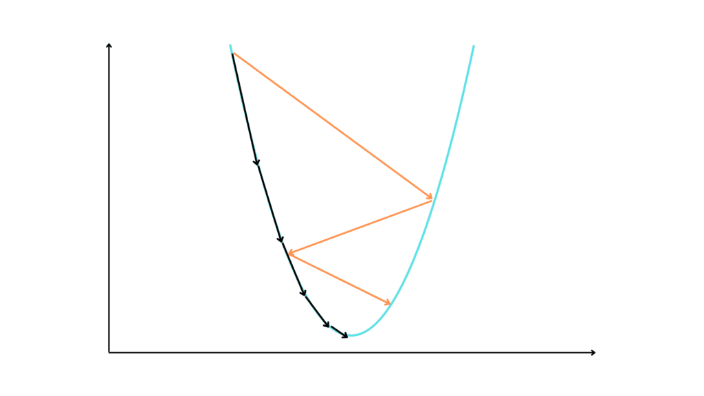
If in adding to x its derivative we increase the value of y, if we subtract from x the derivative we go in the opposite direction, that is, toward the minimum of the function.
The size of the step
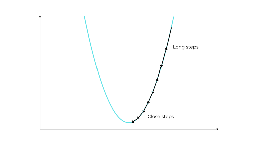
The derivative gives us not only the direction in which to move but also the length of the step.
In fact, at more sloping points of the function, the derivative is greater, and consequently, the y has bigger values. So GD takes longer steps because it knows that the lowest value is far. This allows us to reduce training time.
However, it takes shorter steps at flatter points where the minimum may be close and we need to be cautious and precise.
Gradient descent analogy
Imagine being on a mountain at night and wanting to get down to the valley as quickly as possible. You have at your disposal only a flashlight that allows you to see the ground beneath your feet.
To find the lowest point, you look toward the ascent and take steps in the opposite direction, that is, toward the descent.
If the terrain is very steep you take long steps, knowing you are far from the valley. If the terrain is a little sloping, you take small steps knowing that the lowest point is close.
In this analogy, the mountain is the function and you are the parameter.
Gradient descent limitation
Let’s say we have as input a function like the one in the image.
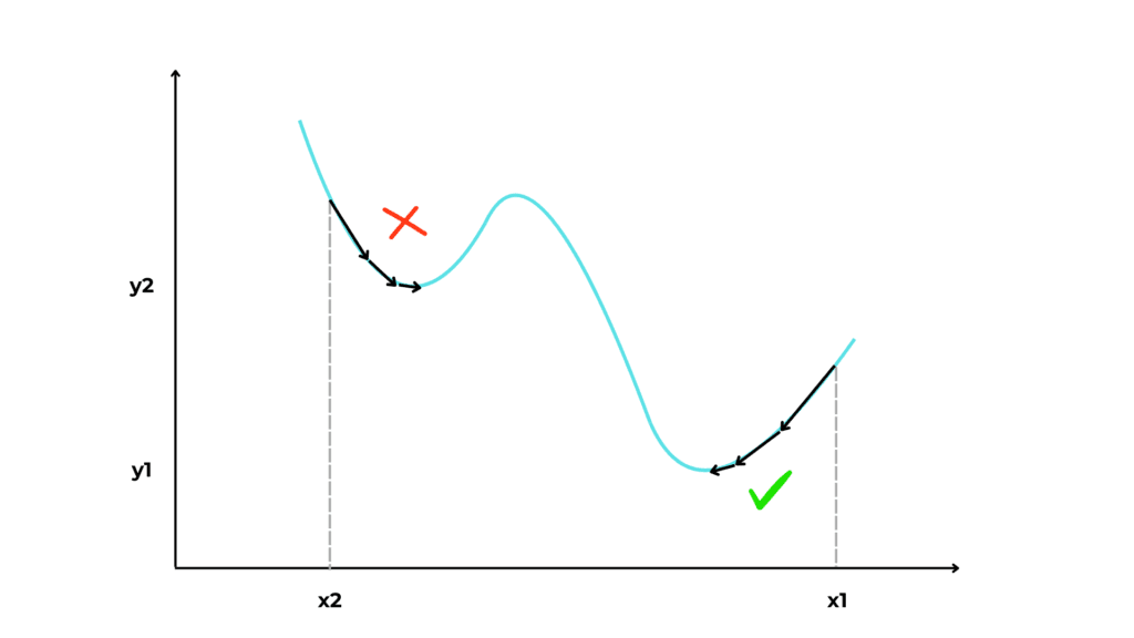
As you can see, if the initial value for x is x1, we successfully reach the lowest point in the function. But if we start from x2, we get to the local minimum in x2 (y2), which is not the global minimum.
Gradient descent types
Batch gradient descent
Batch gradient descent uses all training points at each step to update parameters.
This gives it optimal accuracy but higher computational cost and training time.
Stochastic gradient descent
Stochastic gradient descent uses a random set of training points to update the parameters at each step.
This allows it to have reduced computational cost and training time, but good but not optimal accuracy.